Tutorial for cell-cell communication prediction for non-single-cell ST data with DeepTalk
The notebook introduces to predicting cell-cell comunication using the DeepTalk method.
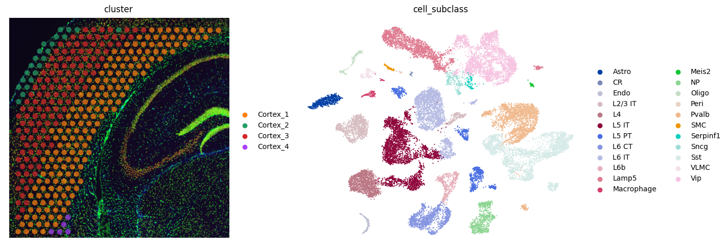
The notebook uses data from mouse brain cortex.
[1]:
import sys
import os
import random
import scanpy as sc
import squidpy as sq
import numpy as np
import pandas as pd
from anndata import AnnData
import pathlib
import matplotlib.pyplot as plt
import matplotlib as mpl
import skimage
import json
import seaborn as sns
import copy
from orderedset import OrderedSet
import DeepTalk_ST as dt
%matplotlib inline
%reload_ext autoreload
%autoreload 2
Loading datasets
Load public data available in Squidpy, from mouse brain cortex. Single cell data are stored in adata_sc. Spatial data, in adata_st..
[2]:
adata_st = sq.datasets.visium_fluo_adata_crop()
adata_st = adata_st[
    adata_st.obs.cluster.isin([f"Cortex_{i}" for i in np.arange(1, 5)])
].copy()
img = sq.datasets.visium_fluo_image_crop()
adata_sc = sq.datasets.sc_mouse_cortex()
[3]:
fig, axs = plt.subplots(1, 2, figsize=(15, 5))
sc.pl.spatial(
    adata_st, color="cluster", alpha=0.7, frameon=False, show=False, ax=axs[0]
)
sc.pl.umap(
    adata_sc, color="cell_subclass", size=10, frameon=False, show=False, ax=axs[1]
)
plt.tight_layout()
Pre-processing
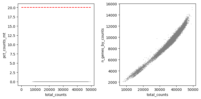
Quality control is applied to single-cell data, as the data has already been preprocessed, this step can be skipped. Different quality control standards should be applied to different data
[4]:
adata_sc.var["mt"] = adata_sc.var_names.str.startswith(r'^(mt-|MT-)')
sc.pp.calculate_qc_metrics(
    adata_sc, qc_vars=["mt"], inplace=True, percent_top=[20], log1p=True
)

fig, axs = plt.subplots(ncols = 2, figsize = (8,4))
sc.pl.scatter(adata_sc, x='total_counts', y='pct_counts_mt',ax = axs[0], show=False)
sc.pl.scatter(adata_sc, x='total_counts', y='n_genes_by_counts',ax = axs[1], show = False)

adata_sc = adata_sc[adata_sc.obs['pct_counts_mt'] < 20]
adata_sc = adata_sc[adata_sc.obs['n_genes_by_counts'] < 16000]
adata_sc = adata_sc[adata_sc.obs['total_counts'] < 55000]

#draw horizontal red lines indicating thresholds.
axs[0].hlines(y = 20, xmin = 0, xmax = max(adata_sc.obs['total_counts']), color = 'red', ls = 'dashed')
fig.tight_layout()
plt.show()
[5]:
sc.pp.filter_cells(adata_sc, min_genes=200)
sc.pp.filter_genes(adata_sc, min_cells=3)
adata_sc_raw = copy.deepcopy(adata_sc)
sc.pp.normalize_total(adata_sc)
sc.pp.log1p(adata_sc)
adata_st_raw = copy.deepcopy(adata_st)
sc.pp.normalize_total(adata_st)
sc.pp.log1p(adata_st)
In order to deconvolve cells, DeepTalk needs to know how many cells are present in each voxel. This is achieved by segmenting the cells on the corresponding histology, which squidpy makes possible with two lines of code: squidpy.im.process applies smoothing as a pre-processing step. - squidpy.im.segment computes segmentation masks with watershed algorithm.
[6]:
sq.im.process(img=img, layer="image", method="smooth")

sq.im.segment(
    img=img,
    layer="image_smooth",
    method="watershed",
    channel=0
)
Let’s visualize the segmentation results for an inset
[7]:
inset_y = 1500
inset_x = 1700
inset_sy = 400
inset_sx = 500

fig, axs = plt.subplots(1, 3, figsize=(30, 10))
sc.pl.spatial(
    adata_st, color="cluster", alpha=0.7, frameon=False, show=False, ax=axs[0], title=""
)
axs[0].set_title("Clusters", fontdict={"fontsize": 20})
sf = adata_st.uns["spatial"]["V1_Adult_Mouse_Brain_Coronal_Section_2"]["scalefactors"][
    "tissue_hires_scalef"
]
rect = mpl.patches.Rectangle(
    (inset_y * sf, inset_x * sf),
    width=inset_sx * sf,
    height=inset_sy * sf,
    ec="yellow",
    lw=4,
    fill=False,
)
axs[0].add_patch(rect)

axs[0].axes.xaxis.label.set_visible(False)
axs[0].axes.yaxis.label.set_visible(False)

axs[1].imshow(
    img["image"][inset_y : inset_y + inset_sy, inset_x : inset_x + inset_sx, 0, 0]
    / 65536,
    interpolation="none",
)
axs[1].grid(False)
axs[1].set_xticks([])
axs[1].set_yticks([])
axs[1].set_title("DAPI", fontdict={"fontsize": 20})

crop = img["segmented_watershed"][
    inset_y : inset_y + inset_sy, inset_x : inset_x + inset_sx
].values.squeeze(-1)
crop = skimage.segmentation.relabel_sequential(crop)[0]
cmap = plt.cm.plasma
cmap.set_under(color="black")
axs[2].imshow(crop, interpolation="none", cmap=cmap, vmin=0.001)
axs[2].grid(False)
axs[2].set_xticks([])
axs[2].set_yticks([])
axs[2].set_title("Nucleous segmentation", fontdict={"fontsize": 20});
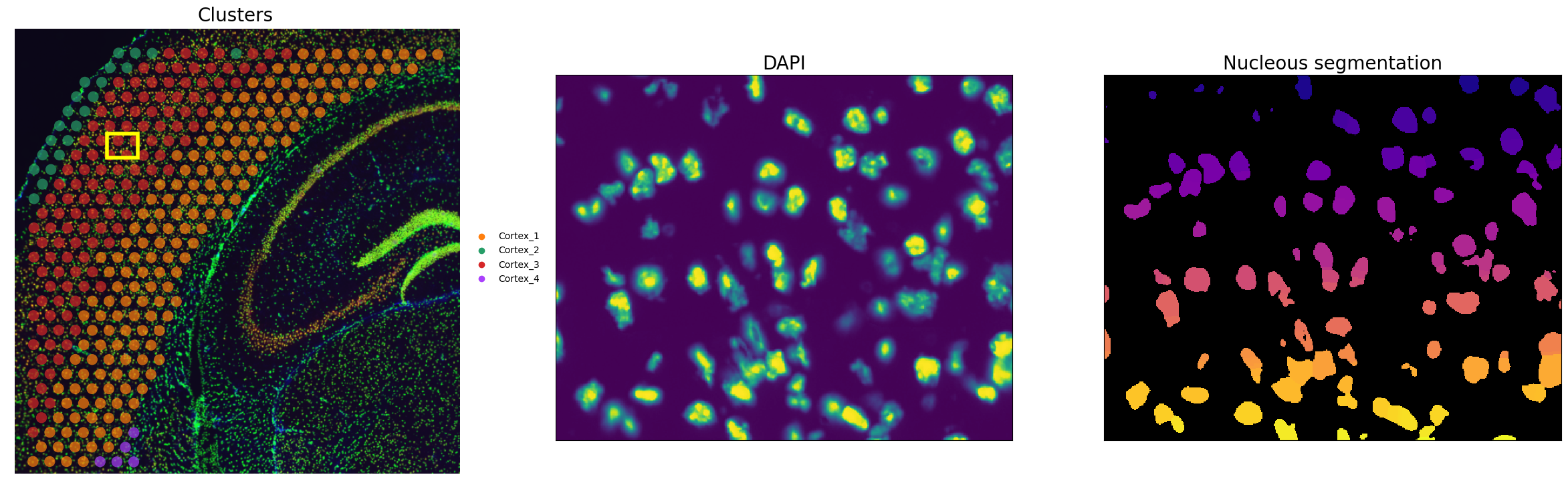
Comparison between DAPI and mask confirms the quality of the segmentation. We then need to extract some image features useful for the deconvolution task downstream. Specifically: - the number of unique segmentation objects (i.e. nuclei) under each spot. - the coordinates of the centroids of the segmentation object.
[8]:
# define image layer to use for segmentation
features_kwargs = {
    "segmentation": {
        "label_layer": "segmented_watershed",
        "props": ["label", "centroid"],
        "channels": [1, 2],
    }
}

sq.im.calculate_image_features(
    adata_st,
    img,
    layer="image",
    key_added="image_features",
    features_kwargs=features_kwargs,
    features="segmentation",
    mask_circle=True,
)
[9]:
adata_st.obsm['image_features']
[9]:
| segmentation_label | segmentation_centroid | |
|---|---|---|
| AAATGGCATGTCTTGT-1 | 13 | [[5304.0, 731.0], [5320.947519118759, 721.3315... |
| AACAACTGGTAGTTGC-1 | 15 | [[1583.0, 4233.828793585227], [1671.5717336342... |
| AACAGGAAATCGAATA-1 | 28 | [[5028.0, 1061.4293230016444], [5042.200781827... |
| AACCCAGAGACGGAGA-1 | 5 | [[1185.0, 1012.0], [1257.9561167460154, 1023.3... |
| AACCGTTGTGTTTGCT-1 | 7 | [[4619.0, 381.72603026366806], [4627.707819057... |
| ... | ... | ... |
| TTGGATTGGGTACCAC-1 | 25 | [[3379.0, 1609.5027775295625], [3430.128033605... |
| TTGGCTCGCATGAGAC-1 | 5 | [[902.0, 3035.1389252487215], [913.41811041094... |
| TTGTATCACACAGAAT-1 | 22 | [[5992.0, 333.5593226506872], [6001.0050156143... |
| TTGTGGCCCTGACAGT-1 | 25 | [[4064.0, 1794.9633829463617], [4082.278586090... |
| TTGTTAGCAAATTCGA-1 | 27 | [[1589.0, 2787.4719677445705], [1597.800292086... |
324 rows × 2 columns
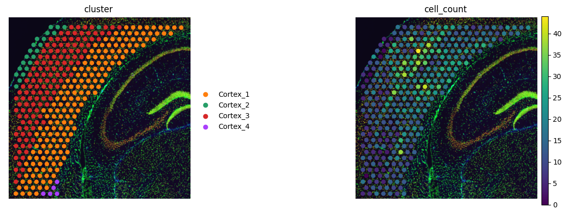
We can visualize the total number of objects under each spot with scanpy.
[10]:
adata_st.obs["cell_count"] = adata_st.obsm["image_features"]["segmentation_label"]
sc.pl.spatial(adata_st, color=["cluster", "cell_count"], frameon=False)
For this case, we use 1291 marker genes as training genes.
[11]:
sc.tl.rank_genes_groups(adata_sc, groupby="cell_subclass", use_raw=False)
markers_df = pd.DataFrame(adata_sc.uns["rank_genes_groups"]["names"]).iloc[0:100, :]
markers = list(np.unique(markers_df.melt().value.values))
len(markers)
WARNING: Default of the method has been changed to 't-test' from 't-test_overestim_var'
[11]:
1291
[12]:
dt.pp_adatas(adata_sc, adata_st, genes=markers)
INFO:root:1187 training genes are saved in `uns``training_genes` of both single cell and spatial Anndatas.
INFO:root:14785 overlapped genes are saved in `uns``overlap_genes` of both single cell and spatial Anndatas.
INFO:root:uniform based density prior is calculated and saved in `obs``uniform_density` of the spatial Anndata.
INFO:root:rna count based density prior is calculated and saved in `obs``rna_count_based_density` of the spatial Anndata.
Deconvolution via DeepTalk
[13]:
ad_map = dt.map_cells_to_space(
    adata_sc=adata_sc,
    adata_sp=adata_st,
    learning_rate=0.0005,
    num_epochs=2000,
    #device='cpu',
    device='cuda:0',
)
Start training
Epoch 100, Loss: -0.683,Score0: 0.683,Time: 0.994
Epoch 200, Loss: -0.688,Score0: 0.688,Time: 0.999
Epoch 300, Loss: -0.691,Score0: 0.691,Time: 1.005
Epoch 400, Loss: -0.694,Score0: 0.694,Time: 1.008
Epoch 500, Loss: -0.697,Score0: 0.697,Time: 1.015
Epoch 600, Loss: -0.700,Score0: 0.700,Time: 1.014
Epoch 700, Loss: -0.702,Score0: 0.702,Time: 1.017
Epoch 800, Loss: -0.705,Score0: 0.705,Time: 1.008
Epoch 900, Loss: -0.708,Score0: 0.708,Time: 1.021
Epoch 1000, Loss: -0.712,Score0: 0.712,Time: 1.017
Epoch 1100, Loss: -0.714,Score0: 0.714,Time: 1.018
Epoch 1200, Loss: -0.718,Score0: 0.718,Time: 1.014
Epoch 1300, Loss: -0.719,Score0: 0.719,Time: 1.015
Epoch 1400, Loss: -0.724,Score0: 0.724,Time: 1.024
Epoch 1500, Loss: -0.726,Score0: 0.726,Time: 1.017
Epoch 1600, Loss: -0.729,Score0: 0.729,Time: 1.019
Epoch 1700, Loss: -0.730,Score0: 0.730,Time: 1.015
Epoch 1800, Loss: -0.732,Score0: 0.732,Time: 1.016
Epoch 1900, Loss: -0.734,Score0: 0.734,Time: 1.015
Epoch 2000, Loss: -0.736,Score0: 0.736,Time: 1.015
[14]:
import torch
torch.cuda.empty_cache()
[15]:
%matplotlib inline
import matplotlib.pyplot as plt
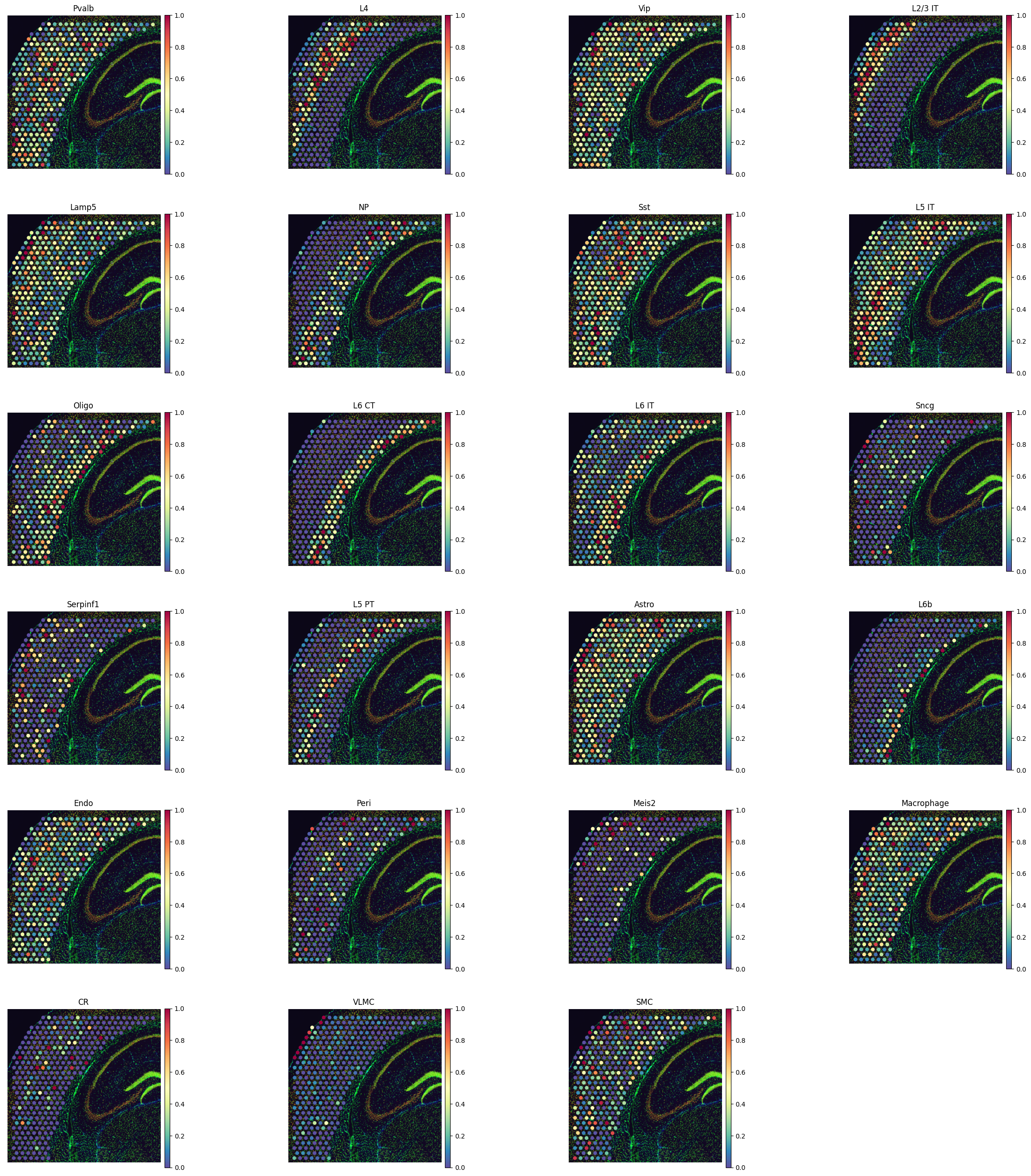
dt.project_cell_annotations(ad_map, adata_st, annotation="cell_subclass")
annotation_list = list(pd.unique(adata_sc.obs['cell_subclass']))
dt.plot_cell_annotation_sc1(adata_st, annotation_list,perc=0.02, cmap='Spectral_r', ncols=4,
                           scale_factor=adata_st.uns['spatial']['V1_Adult_Mouse_Brain_Coronal_Section_2']['scalefactors']['tissue_hires_scalef'])
INFO:root:spatial prediction dataframe is saved in `obsm` `tangram_ct_pred` of the spatial AnnData.
<Figure size 640x480 with 0 Axes>
[16]:
ad_ge = dt.project_genes(adata_map=ad_map, adata_sc=adata_sc)
ad_ge
[16]:
AnnData object with n_obs × n_vars = 324 × 36826
    obs: 'in_tissue', 'array_row', 'array_col', 'n_genes_by_counts', 'log1p_n_genes_by_counts', 'total_counts', 'log1p_total_counts', 'pct_counts_in_top_50_genes', 'pct_counts_in_top_100_genes', 'pct_counts_in_top_200_genes', 'pct_counts_in_top_500_genes', 'total_counts_MT', 'log1p_total_counts_MT', 'pct_counts_MT', 'n_counts', 'leiden', 'cluster', 'cell_count', 'uniform_density', 'rna_count_based_density'
    var: 'mt', 'n_cells_by_counts', 'mean_counts', 'log1p_mean_counts', 'pct_dropout_by_counts', 'total_counts', 'log1p_total_counts', 'n_cells', 'highly_variable', 'highly_variable_rank', 'means', 'variances', 'variances_norm', 'sparsity', 'is_training'
    uns: 'cell_class_colors', 'cell_subclass_colors', 'hvg', 'neighbors', 'pca', 'umap', 'log1p', 'rank_genes_groups', 'training_genes', 'overlap_genes'
[17]:
ad_ge.uns['spatial'] = adata_st.uns['spatial'].copy()
ad_ge.obsm['spatial'] = adata_st.obsm['spatial'].copy()
[18]:
df_all_genes = dt.compare_spatial_geneexp(ad_ge, adata_st, adata_sc)
df_all_genes
[18]:
| score | is_training | sparsity_sp | sparsity_sc | sparsity_diff | |
|---|---|---|---|---|---|
| hspa8 | 9.975005e-01 | True | 0.000000 | 0.000784 | -0.000784 |
| ppia | 9.972653e-01 | True | 0.000000 | 0.000092 | -0.000092 |
| gapdh | 9.972501e-01 | True | 0.000000 | 0.000968 | -0.000968 |
| atp1b1 | 9.972034e-01 | False | 0.000000 | 0.014334 | -0.014334 |
| tmsb4x | 9.970869e-01 | True | 0.000000 | 0.002811 | -0.002811 |
| ... | ... | ... | ... | ... | ... |
| irx5 | 1.419255e-06 | False | 0.996914 | 0.999447 | -0.002533 |
| cutal | 3.581884e-07 | False | 0.996914 | 0.997696 | -0.000782 |
| 1810010k12rik | 7.292536e-08 | False | 0.996914 | 0.999585 | -0.002672 |
| dmrt3 | 1.533246e-08 | False | 0.996914 | 0.999263 | -0.002349 |
| gm15133 | 2.075689e-09 | False | 0.996914 | 0.999170 | -0.002257 |
14785 rows × 5 columns
[19]:
dt.create_segment_cell_df(adata_st)
#adata_st.uns["tangram_cell_segmentation"]
[20]:
dt.count_cell_annotations(
    ad_map,
    adata_sc,
    adata_st,
    annotation="cell_subclass",
)
#adata_st.obsm["tangram_ct_count"]
[21]:
adata_segment = dt.deconvolve_cell_annotations(adata_st)
#adata_segment.obs
[22]:
mapping_colors = {
    "L6_CT": (0.19215686274509805, 0.5098039215686274, 0.7411764705882353),
    "L6_IT": (0.4196078431372549, 0.6823529411764706, 0.8392156862745098),
    "NP": (0.6196078431372549, 0.792156862745098, 0.8823529411764706),
    "L6b": "#0000c2ff",
    "L2/3_IT": "#a1ed7bff",
    "L5_IT": (0.19215686274509805, 0.6392156862745098, 0.32941176470588235),
    "L5_ET": (0.4549019607843137, 0.7686274509803922, 0.4627450980392157),
    "Oligo": (0.4588235294117647, 0.4196078431372549, 0.6941176470588235),
    "Vip": (0.6196078431372549, 0.6039215686274509, 0.7843137254901961),
    "Astro": "#ffdd55ff",
    "L6_CT": "#000000ff",
    "Pvalb": (0.38823529411764707, 0.38823529411764707, 0.38823529411764707),
    "Lamp5": (0.5882352941176471, 0.5882352941176471, 0.5882352941176471),
    "Sst": (0.7411764705882353, 0.7411764705882353, 0.7411764705882353),
    "CR": (0.8509803921568627, 0.8509803921568627, 0.8509803921568627),
    "Sncg": (0.5176470588235295, 0.23529411764705882, 0.2235294117647059),
    "Peri": (0.6784313725490196, 0.28627450980392155, 0.2901960784313726),
    "VLMC": (0.8392156862745098, 0.3803921568627451, 0.4196078431372549),
    "Endo": (0.9058823529411765, 0.5882352941176471, 0.611764705882353),
    "Meis2": "#FFA500ff",
    "SMC": "#000000ff",
    "L6_PT": "#4682B4ff",
    "L5_PT": (0.19215686274509805, 0.6392156862745098, 0.32941176470588235),
    "L5_NP": "#6B8E23ff",
    "L4": "#d61f1dff",
    "Macrophage": "#2b2d2fff",
    "Serpinf1": "#000000ff",
}
[23]:
newmeta = adata_segment.obs.copy()
newmeta.columns = newmeta.columns.str.replace(".", "-")
newmeta.insert(0, 'cell', newmeta.index)
newmeta["cell"] = newmeta["cell"].astype(int) + 1
newmeta["cell"] = "C" + newmeta["cell"].astype(str)
newmeta['spot'] = newmeta['centroids'].apply(lambda x: x.split('_')[0])
newmeta.rename(columns={'cluster': 'celltype'}, inplace=True)
newmeta["celltype"] = newmeta["celltype"].str.replace(" ", "_")
meta_data = newmeta[['cell','x','y','celltype']]
[24]:
%matplotlib inline
import matplotlib.pyplot as plt
cluster = meta_data['celltype'].values
new_column_names = {'x': 'y', 'y': 'x'}
adata_segment.obs = adata_segment.obs.rename(columns=new_column_names)
dt.plot_cell_type_ST(adata_segment,mapping_colors,cluster)

Prediction of spatial CCC at the single-cell resolution.
Train the data using subgraph-based GAT and generate a prediction model.
The training process may take some time.
The trained model can be used to predict intercellular communication mediated by other L-R interactions
[25]:
Test_dir = './test/spot/'
isExists = os.path.exists(Test_dir)
if isExists:
    pass
else:
    os.makedirs(Test_dir)
[26]:
index1 = [word.capitalize() for word in adata_sc.var.index]
c_list = [f'C{i}' for i in range(1, adata_sc.X.shape[0]+1)]
ad_sc = pd.DataFrame(adata_sc.X.T,index=index1,columns=c_list)

index1 = [word.capitalize() for word in ad_ge.var.index]
c_list = [word.capitalize() for word in ad_ge.obs.index]
ad_ge_new = pd.DataFrame(ad_ge.X.T,index=index1,columns=c_list)
st_obs = adata_segment.obs.copy()
sc_obs = adata_sc.obs.copy()
[27]:
stnewdata = dt.New_ST_data_pre(ad_sc, ad_ge_new, st_obs, sc_obs, outdir = Test_dir)
[28]:
pathways = Test_dir + "/pathways.csv"
#lrpairs = Test_dir + "/lrpairs_new.csv"
st_data = stnewdata
species = "Mouse"
Generate training data.
[29]:
lrpairs_train = {
    'ligand': ['Mif'],
    'receptor': ['Epha5'],
    'species': ['Mouse']
}

lrpairs_train = pd.DataFrame(lrpairs_train)
lrpairs_train
[29]:
| ligand | receptor | species | |
|---|---|---|---|
| 0 | Mif | Epha5 | Mouse |
[30]:
dt.File_Train(st_data, pathways, lrpairs_train, meta_data, species, LR_train = 'Mif_Epha5',
              outdir =  Test_dir)
[31]:
dt.data_for_train(st_data, data_dir = Test_dir +'/data/',
    LR_train = 'Mif_Epha5')
The process will take a long time, but we provide pre-trained models, so you can choose to skip this step.
[32]:
dt.Train(data_name = 'Mif_Epha5', data_path = Test_dir + '/data/',
    outdir = Test_dir + '/data/Mif_Epha5/output',
    pretrained_embeddings = Test_dir + '/data/Mif_Epha5/data_pca.emd',
    n_epochs = 50,ft_n_epochs=10)
 Loading graph...
DataSet Stats :
Number of Nodes 5044
Number of Edges 61086
Number of Node types 1
Number of relations 1
Graph with 5044 nodes and 61086 edges
5044 2
check torch.Size([5044, 128]) 5020
node2vec tensor torch.Size([5044, 128])
No. of nodes with pretrained embedding:  5044
No. edges in test data:  22942
***************PRETRAINING***************

 generate walks ...
no. of walks 40352
train ./test/spot//data//Mif_Epha5/outdir/Mif_Epha5_walks_train.txt
validate ./test/spot//data//Mif_Epha5/outdir/Mif_Epha5_walks_validate.txt
test ./test/spot//data//Mif_Epha5/outdir/Mif_Epha5_walks_test.txt

 Run model for pre-training ...

 Begin Training

Epoch: 0
MinLoss: 1000000.0, CurLoss: 8.6501
epoch time: (s) 68.51210856437683

Epoch: 10
MinLoss: 1000000.0, CurLoss: 8.4105
epoch time: (s) 64.37373161315918

Epoch: 20
MinLoss: 1000000.0, CurLoss: 7.8265
epoch time: (s) 66.30228304862976

Epoch: 30
MinLoss: 1000000.0, CurLoss: 7.1092
epoch time: (s) 63.97214436531067

Epoch: 40
MinLoss: 1000000.0, CurLoss: 6.3965
epoch time: (s) 65.09792852401733

Best Epoch: 49
In GenericGraph link Prediction Generation
80298
Generating false edges by random false target
train
valid
test

 !!!!
4 4 Linear(in_features=512, out_features=512, bias=True)
Evaluating valid batch 0
Evaluating valid batch 100
Evaluating test batch 0
Evaluating test batch 100
Evaluating test batch 200

 Begin evaluation for link prediction...
----------------------In run_evaluation_main()------------
y_true.shape: (267725,), y_scores.shape: (267725,), y_pred.shape: (267725,)
workflow2 : ROC-AUC: 0.5046388546686829, F1: 0.9460243646325961, AUC: 0.9264366885093068

Evaluation by edge type:
Performance on edge type:  to
y_true.shape: (22942,), y_scores.shape: (22942,), y_pred.shape: (22942,)
workflow2 : ROC-AUC: 0.507387220336155, F1: 0.9464734210465678, PR-AUC: 0.9269457355309407
END
***************FINETUNING***************

 Run model for finetuning ...
4 4 Linear(in_features=512, out_features=512, bias=True)

 Begin Training
MinLoss: 1000000.0, CurLoss: 0.2287
MinLoss: 0.2287, CurLoss: 0.225

Finetune epoch:  0
MinLoss:  0.225
epoch time: (s) 814.3929345607758
MinLoss: 1000000.0, CurLoss: 0.2167
MinLoss: 0.2167, CurLoss: 0.2095

Finetune epoch:  1
MinLoss:  0.2095
epoch time: (s) 824.5920221805573
MinLoss: 1000000.0, CurLoss: 0.2085
MinLoss: 0.2085, CurLoss: 0.2066

Finetune epoch:  2
MinLoss:  0.2066
epoch time: (s) 817.0912182331085
MinLoss: 1000000.0, CurLoss: 0.2087
MinLoss: 0.2087, CurLoss: 0.207

Finetune epoch:  3
MinLoss:  0.207
epoch time: (s) 817.972235918045
MinLoss: 1000000.0, CurLoss: 0.2102
MinLoss: 0.2102, CurLoss: 0.2073

Finetune epoch:  4
MinLoss:  0.2073
epoch time: (s) 825.3906593322754
MinLoss: 1000000.0, CurLoss: 0.2107
MinLoss: 0.2107, CurLoss: 0.2092

Finetune epoch:  5
MinLoss:  0.2092
epoch time: (s) 821.301789522171
MinLoss: 1000000.0, CurLoss: 0.212
MinLoss: 0.212, CurLoss: 0.2107

Finetune epoch:  6
MinLoss:  0.2107
epoch time: (s) 831.1592559814453
MinLoss: 1000000.0, CurLoss: 0.2131
MinLoss: 0.2131, CurLoss: 0.2145

Finetune epoch:  7
MinLoss:  0.2131
epoch time: (s) 826.9757378101349
MinLoss: 1000000.0, CurLoss: 0.2146
MinLoss: 0.2146, CurLoss: 0.2162

Finetune epoch:  8
MinLoss:  0.2146
epoch time: (s) 823.7158391475677
MinLoss: 1000000.0, CurLoss: 0.2181
MinLoss: 0.2181, CurLoss: 0.2196

Finetune epoch:  9
MinLoss:  0.2181
epoch time: (s) 821.5212824344635

Best Epoch: 2
Begin Testing
4 4 Linear(in_features=512, out_features=512, bias=True)
4 4 Linear(in_features=512, out_features=512, bias=True)
Evaluating test batch 0
Evaluating test batch 100
Evaluating test batch 200

 Begin evaluation for link prediction...
----------------------In run_evaluation_main()------------
y_true.shape: (267725,), y_scores.shape: (267725,), y_pred.shape: (267725,)
workflow3 : ROC-AUC: 0.878169012719133, F1: 0.952280316840628, AUC: 0.9878695217128189

Evaluation by edge type:
Performance on edge type:  to
y_true.shape: (22942,), y_scores.shape: (22942,), y_pred.shape: (22942,)
workflow3 : ROC-AUC: 0.8785313540392228, F1: 0.952613879547539, PR-AUC: 0.9877795008274386
END
running time(seconds) on Mif_Epha5 data: 13920.463974237442
Generate prediction data for Sema3c-Fzd3 pair.
[33]:
lrpairs_pre = {
    'ligand': ['Sema3c'],
    'receptor': ['Fzd3'],
    'species': ['Mouse']
}

lrpairs_pre = pd.DataFrame(lrpairs_pre)
lrpairs_pre
[33]:
| ligand | receptor | species | |
|---|---|---|---|
| 0 | Sema3c | Fzd3 | Mouse |
[34]:
dt.File_Pre(st_data, pathways, lrpairs_pre, meta_data, species, LR_Pre = 'Sema3c_Fzd3',
              outdir =  Test_dir)
[35]:
dt.data_for_pre(st_data, data_dir = Test_dir +'/data/',
    LR_pre = 'Sema3c_Fzd3')
Predicting cell-cell communication mediated by ``Sema3c_Fzd3``.
[36]:
dt.run_predict(data_name='Sema3c_Fzd3',data_path = Test_dir +'/data/',
    outdir = Test_dir +'/data/Sema3c_Fzd3/output',
    pretrained_embeddings = Test_dir +'/data/Sema3c_Fzd3/data_pca_test.emd',
    model_path = Test_dir+'/data/Mif_Epha5/output/finetune/results',best_id = 2,
    is_trained = True, model_name = Test_dir + '/Mif_Epha5.model'
    )
DataSet Stats :
Number of Nodes 4624
Number of Edges 32577
Number of Node types 1
Number of relations 1
check torch.Size([4624, 128]) 4085
node2vec tensor torch.Size([4624, 128])
4 4 Linear(in_features=512, out_features=512, bias=True)
Begin Predicting
Done
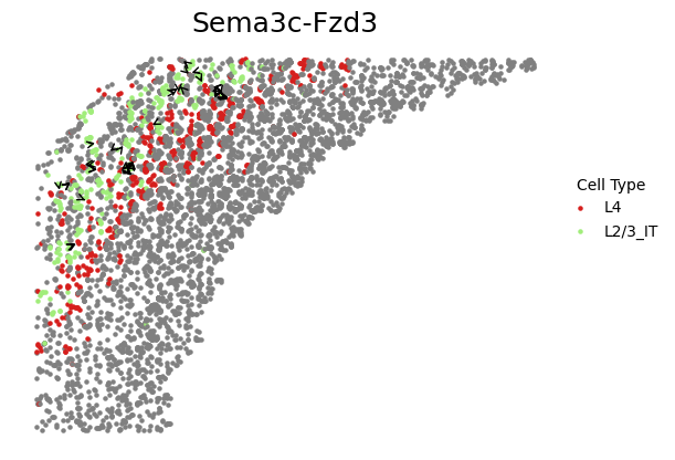
Visualize of the spatial CCC
[37]:
%matplotlib inline
import matplotlib.pyplot as plt

dt.plot_CCC_ST(adata_segment, mapping_colors, cluster, st_data, ligand = 'Sema3c',
    receptor = 'Fzd3',CCC_label = Test_dir + '/data/Sema3c_Fzd3/predict_ccc.txt',
    sourcetype = 'L2/3_IT',targettype = 'L4',top_score = 50)
[38]:
%matplotlib inline
import matplotlib.pyplot as plt
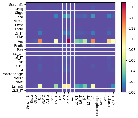
dt.plot_CCC_heatmap(cluster, st_data, ligand = 'Sema3c', receptor = 'Fzd3',
    CCC_label = Test_dir + '/data/Sema3c_Fzd3/predict_ccc.txt')
[ ]: