Tutorial for cell-cell communication prediction for single-ST data with DeepTalk
The notebook introduces to predicting cell-cell comunication using the DeepTalk method.
The notebook uses data from mouse brain cortex.
Installation
Make sure DeepTalk_ST is installed via pip install DeepTalk_ST.
The Python environment needs to install the packages listed in environment.yml.
[1]:
import sys
import os
import random
import scanpy as sc
import squidpy as sq
import numpy as np
import pandas as pd
from anndata import AnnData
import pathlib
import matplotlib.pyplot as plt
import matplotlib as mpl
import skimage
import json
import seaborn as sns
import copy
from orderedset import OrderedSet
import DeepTalk_ST as dt

%reload_ext autoreload
%autoreload 2
%matplotlib inline
Create a work folder and Download the data
The MERFISH_genes.csv, st_flie.txt, st_location.txt, single_cell_process.R, geneinfo.rda,pathways.rda, lrpairs_new.csv, df_pathways.csv can be downloaded from https://github.com/JiangBioLab/DeepTalk/tree/main/test.
[2]:
Test_dir = './test/single-cell/'
isExists = os.path.exists(Test_dir)
if isExists:
    pass
else:
    os.makedirs(Test_dir)
[3]:
'''
# Skip this cells if data are already downloaded
!wget http://jianglab.org.cn/deeptalk_download/visp_sn_tpm_small_0430.tar.gz -O ./Test1/single-cell/visp_sn_tpm_small_0430.tar.gz
!tar -xzvf visp_sn_tpm_small_0430.tar.gz -C Test_dir
'''
[3]:
'\n# Skip this cells if data are already downloaded\n!wget http://jianglab.org.cn/deeptalk_download/visp_sn_tpm_small_0430.tar.gz -O ./Test1/single-cell/visp_sn_tpm_small_0430.tar.gz\n!tar -xzvf visp_sn_tpm_small_0430.tar.gz -C Test_dir\n'
Load spatial data
Spatial data need to be organized as a voxel-by-gene matrix. Here, MERFISH data contains 2,399 spatial voxels, in each of which there are 268 genes measured.
[4]:
random.seed(1000)
ad_st = sc.read_csv(Test_dir + "/st_flie.txt", delimiter='\t', first_column_names=True)
ad_st
[4]:
AnnData object with n_obs × n_vars = 2399 × 268
[5]:
ad_st_raw = copy.deepcopy(ad_st)
#ad_st_raw = ad_st
sc.pp.normalize_total(ad_st)
#ad_st_raw1 = copy.deepcopy(ad_st)
#sc.pp.normalize_per_cell(ad_st, counts_per_cell_after=1e4)
sc.pp.log1p(ad_st)
[6]:
st_spatial = np.loadtxt(Test_dir + "/st_location.txt",dtype=str, delimiter=' ')
st_spatial = st_spatial.astype(np.float64)
[7]:
ad_st.obs['x'] = st_spatial[:,0]
ad_st.obs['y'] = st_spatial[:,1]
ad_st.obsm["spatial"]=st_spatial
ad_st_raw.obsm["spatial"]=st_spatial
[8]:
ad_st.obs.copy()
[8]:
| x | y | |
|---|---|---|
| 0 | 1161.113371 | 6178.383054 |
| 1 | 1162.913371 | 6113.133054 |
| 2 | 1168.313371 | 6046.083054 |
| 3 | 1163.813371 | 6202.683054 |
| 4 | 1166.963371 | 6083.883054 |
| ... | ... | ... |
| 2394 | 3144.263371 | 5201.433054 |
| 2395 | 3154.613371 | 5331.033054 |
| 2396 | 3165.413371 | 5190.183054 |
| 2397 | 3189.713371 | 5292.783054 |
| 2398 | 3196.913371 | 5196.933054 |
2399 rows × 2 columns
[9]:
xs = ad_st.obs.x.values
ys = ad_st.obs.y.values
plt.axis('off')
plt.scatter(xs, ys, s=.7);
plt.gca().invert_yaxis()
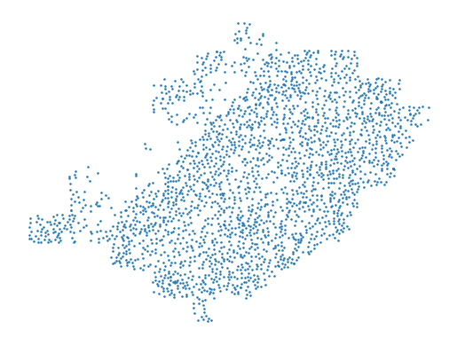
Single cell data
By single cell data, we generally mean either scRNAseq or snRNAseq. They are 11,759 SMART-Seq2 snRNA-seq data from the VISp region.
[10]:
path = os.path.join(Test_dir + "/visp_sn_tpm_small_0430.h5ad")
ad_sc = sc.read_h5ad(path)
[11]:
ad_sc
[11]:
AnnData object with n_obs × n_vars = 11759 × 40056
    obs: 'consensus_cluster', 'reference_cluster', 'reference_color', 'broad_class', 'subclass', 'merged_cluster_smFISH', 'merged_cluster_ISS', 'total_reads', 'cpm_scaling_factor', 'n_genes'
    var: 'length', 'maxMeanFpkm', 'in_MERFISH', 'gene_id', 'chromosome', 'gene_entrez_id', 'gene_name', 'n_cells'
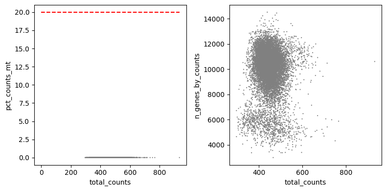
Quality control is applied to single-cell data, as the data has already been preprocessed, this step can be skipped. Different quality control standards should be applied to different data
[12]:
ad_sc.var["mt"] = ad_sc.var_names.str.startswith(r'^(mt-|MT-)')
sc.pp.calculate_qc_metrics(
    ad_sc, qc_vars=["mt"], inplace=True, percent_top=[20], log1p=True
)


fig, axs = plt.subplots(ncols = 2, figsize = (8,4))
sc.pl.scatter(ad_sc, x='total_counts', y='pct_counts_mt',ax = axs[0], show=False)
sc.pl.scatter(ad_sc, x='total_counts', y='n_genes_by_counts',ax = axs[1], show = False)

ad_sc = ad_sc[ad_sc.obs['pct_counts_mt'] < 20]
ad_sc = ad_sc[ad_sc.obs['n_genes_by_counts'] < 15000]
ad_sc = ad_sc[ad_sc.obs['total_counts'] < 1000]

#draw horizontal red lines indicating thresholds.
axs[0].hlines(y = 20, xmin = 0, xmax = max(ad_sc.obs['total_counts']), color = 'red', ls = 'dashed')
fig.tight_layout()
plt.show()
[13]:
sc.pp.filter_cells(ad_sc, min_genes=200)
sc.pp.filter_genes(ad_sc, min_cells=3)
ad_sc_raw0 = copy.deepcopy(ad_sc)
sc.pp.normalize_total(ad_sc)
#sc.pp.normalize_per_cell(ad_sc, counts_per_cell_after=1e4)
ad_sc_raw1 = copy.deepcopy(ad_sc)
sc.pp.log1p(ad_sc)
ad_sc_raw = copy.deepcopy(ad_sc)
sc.pp.highly_variable_genes(ad_sc, min_mean=0.0125, max_mean=4, min_disp=0.25)
sc.pp.scale(ad_sc, max_value=10)
ad_sc_raw2 = copy.deepcopy(ad_sc)
sc.pp.pca(ad_sc)
sc.pp.neighbors(ad_sc)
sc.tl.umap(ad_sc)
ad_sc
[13]:
AnnData object with n_obs × n_vars = 11759 × 40056
    obs: 'consensus_cluster', 'reference_cluster', 'reference_color', 'broad_class', 'subclass', 'merged_cluster_smFISH', 'merged_cluster_ISS', 'total_reads', 'cpm_scaling_factor', 'n_genes', 'n_genes_by_counts', 'log1p_n_genes_by_counts', 'total_counts', 'log1p_total_counts', 'pct_counts_in_top_20_genes', 'total_counts_mt', 'log1p_total_counts_mt', 'pct_counts_mt'
    var: 'length', 'maxMeanFpkm', 'in_MERFISH', 'gene_id', 'chromosome', 'gene_entrez_id', 'gene_name', 'n_cells', 'mt', 'n_cells_by_counts', 'mean_counts', 'log1p_mean_counts', 'pct_dropout_by_counts', 'total_counts', 'log1p_total_counts', 'highly_variable', 'means', 'dispersions', 'dispersions_norm', 'mean', 'std'
    uns: 'log1p', 'hvg', 'pca', 'neighbors', 'umap'
    obsm: 'X_pca', 'X_umap'
    varm: 'PCs'
    obsp: 'distances', 'connectivities'
[14]:
ad_sc_raw.obsm['X_umap']=ad_sc.obsm['X_umap']
Prepare to integration
[15]:
df_genes = pd.read_csv(Test_dir + '/MERFISH_genes.csv',header=None)
markers = np.reshape(df_genes.values[:,-1], (-1, ))
markers = list(markers)
len(markers)
[15]:
254
[16]:
dt.pp_adatas(ad_sc_raw, ad_st, genes=markers)
INFO:root:253 training genes are saved in `uns``training_genes` of both single cell and spatial Anndatas.
INFO:root:257 overlapped genes are saved in `uns``overlap_genes` of both single cell and spatial Anndatas.
INFO:root:uniform based density prior is calculated and saved in `obs``uniform_density` of the spatial Anndata.
INFO:root:rna count based density prior is calculated and saved in `obs``rna_count_based_density` of the spatial Anndata.
Integration sc/snRNA-seq and ST data
[17]:
ad_map = dt.map_cells_to_space(
    adata_sc=ad_sc_raw,
    adata_sp=ad_st,
    learning_rate=0.0001,
    num_epochs=3000,
    device='cuda:0',
)
Start training
Epoch 100, Loss: -0.529,Score0: 0.529,Time: 0.106
Epoch 200, Loss: -0.563,Score0: 0.563,Time: 0.100
Epoch 300, Loss: -0.589,Score0: 0.589,Time: 0.103
Epoch 400, Loss: -0.608,Score0: 0.608,Time: 0.102
Epoch 500, Loss: -0.622,Score0: 0.622,Time: 0.108
Epoch 600, Loss: -0.634,Score0: 0.634,Time: 0.102
Epoch 700, Loss: -0.642,Score0: 0.642,Time: 0.102
Epoch 800, Loss: -0.650,Score0: 0.650,Time: 0.103
Epoch 900, Loss: -0.656,Score0: 0.656,Time: 0.100
Epoch 1000, Loss: -0.662,Score0: 0.662,Time: 0.101
Epoch 1100, Loss: -0.667,Score0: 0.667,Time: 0.105
Epoch 1200, Loss: -0.672,Score0: 0.672,Time: 0.102
Epoch 1300, Loss: -0.677,Score0: 0.677,Time: 0.103
Epoch 1400, Loss: -0.681,Score0: 0.681,Time: 0.106
Epoch 1500, Loss: -0.685,Score0: 0.685,Time: 0.102
Epoch 1600, Loss: -0.689,Score0: 0.689,Time: 0.102
Epoch 1700, Loss: -0.692,Score0: 0.692,Time: 0.101
Epoch 1800, Loss: -0.696,Score0: 0.696,Time: 0.102
Epoch 1900, Loss: -0.699,Score0: 0.699,Time: 0.103
Epoch 2000, Loss: -0.702,Score0: 0.702,Time: 0.101
Epoch 2100, Loss: -0.704,Score0: 0.704,Time: 0.104
Epoch 2200, Loss: -0.707,Score0: 0.707,Time: 0.102
Epoch 2300, Loss: -0.709,Score0: 0.709,Time: 0.104
Epoch 2400, Loss: -0.711,Score0: 0.711,Time: 0.103
Epoch 2500, Loss: -0.713,Score0: 0.713,Time: 0.107
Epoch 2600, Loss: -0.715,Score0: 0.715,Time: 0.101
Epoch 2700, Loss: -0.717,Score0: 0.717,Time: 0.100
Epoch 2800, Loss: -0.719,Score0: 0.719,Time: 0.108
Epoch 2900, Loss: -0.721,Score0: 0.721,Time: 0.106
Epoch 3000, Loss: -0.722,Score0: 0.722,Time: 0.107
[18]:
import torch
torch.cuda.empty_cache()
[19]:
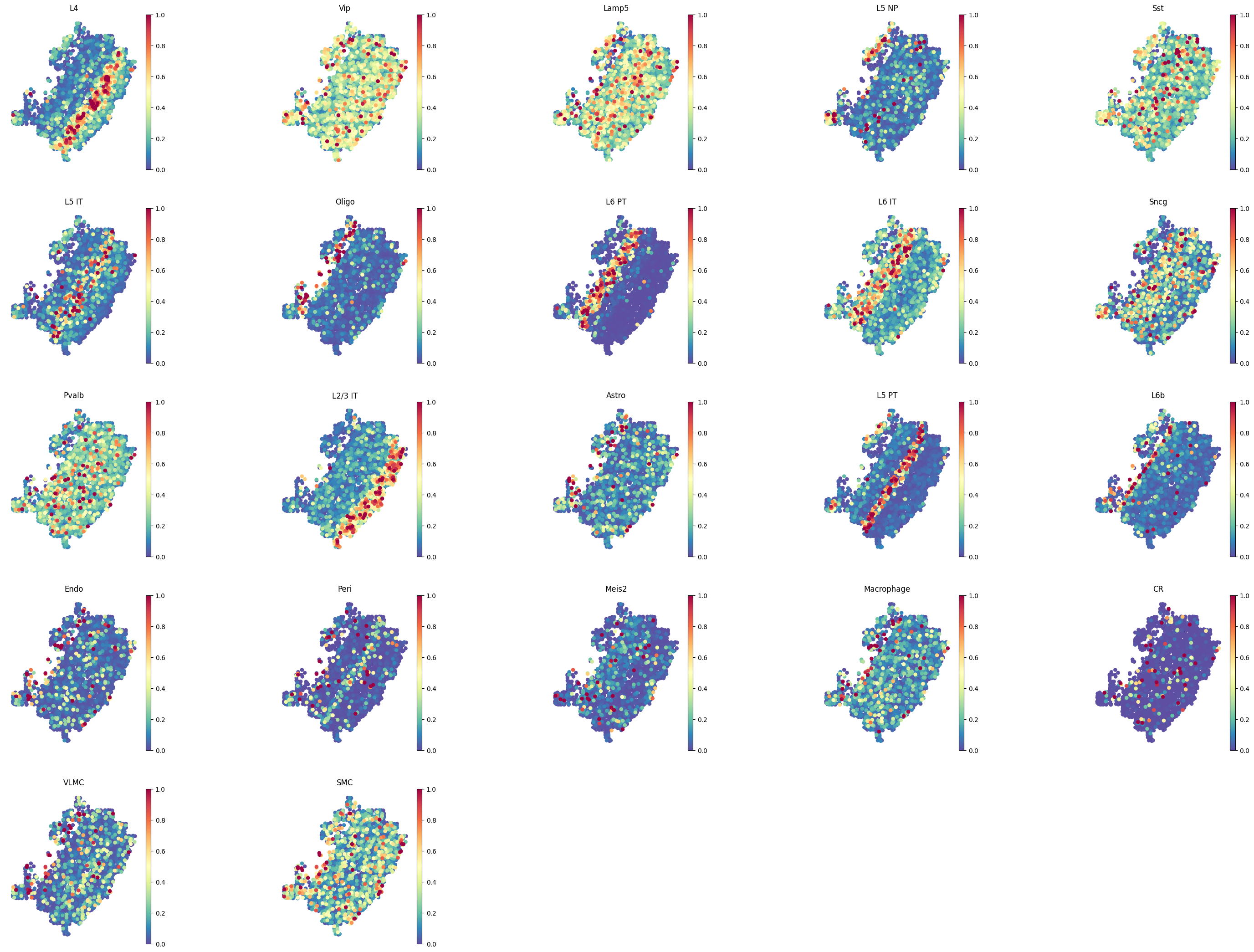
dt.project_cell_annotations(ad_map, ad_st, annotation="subclass")
annotation_list = list(pd.unique(ad_sc_raw.obs['subclass']))
dt.plot_cell_annotation_sc1(ad_st, annotation_list,spot_size=65, ncols=5,cmap='Spectral_r', scale_factor=0.1,perc=0.01)
INFO:root:spatial prediction dataframe is saved in `obsm` `tangram_ct_pred` of the spatial AnnData.
<Figure size 640x480 with 0 Axes>
Prepare to inference of cell-cell communication
[20]:
gene_all_mouse, gene_all_human = dt.gene_select(lrpairs = Test_dir + '/lrpairs_new.csv',TF = Test_dir + '/df_pathways.csv')
[21]:
ad_ge = dt.project_genes(adata_map=ad_map, adata_sc=ad_sc_raw)
ad_ge
[21]:
AnnData object with n_obs × n_vars = 2399 × 40056
    obs: 'x', 'y', 'uniform_density', 'rna_count_based_density'
    var: 'length', 'maxMeanFpkm', 'in_MERFISH', 'gene_id', 'chromosome', 'gene_entrez_id', 'gene_name', 'n_cells', 'mt', 'n_cells_by_counts', 'mean_counts', 'log1p_mean_counts', 'pct_dropout_by_counts', 'total_counts', 'log1p_total_counts', 'sparsity', 'is_training'
    uns: 'log1p', 'training_genes', 'overlap_genes'
[22]:
sc.pp.filter_cells(ad_ge, min_genes=200)
sc.pp.filter_genes(ad_ge, min_cells=3)
sc.pp.filter_genes_dispersion(ad_ge, flavor='cell_ranger', log=False)
ad_ge = ad_ge[:, ad_ge.X.mean(axis=0) >= 0.1]
ad_ge
[22]:
View of AnnData object with n_obs × n_vars = 2399 × 2051
    obs: 'x', 'y', 'uniform_density', 'rna_count_based_density', 'n_genes'
    var: 'length', 'maxMeanFpkm', 'in_MERFISH', 'gene_id', 'chromosome', 'gene_entrez_id', 'gene_name', 'n_cells', 'mt', 'n_cells_by_counts', 'mean_counts', 'log1p_mean_counts', 'pct_dropout_by_counts', 'total_counts', 'log1p_total_counts', 'sparsity', 'is_training', 'means', 'dispersions', 'dispersions_norm'
    uns: 'log1p', 'training_genes', 'overlap_genes'
[23]:
index1 = [word.capitalize() for word in ad_ge.var.index]
c_list = [f'C{i}' for i in range(1, ad_ge.X.shape[0]+1)]
st_data = pd.DataFrame(ad_ge.X.T,index=index1,columns=c_list)
st_data = st_data[st_data.index.isin(gene_all_mouse)]
#st_data.to_csv(Test_dir + '/ad_st_test.csv')
#df.to_csv(Test_dir + '/ad_st_test.csv',float_format='%.2f')
st_data
[23]:
| C1 | C2 | C3 | C4 | C5 | C6 | C7 | C8 | C9 | C10 | ... | C2390 | C2391 | C2392 | C2393 | C2394 | C2395 | C2396 | C2397 | C2398 | C2399 | |
|---|---|---|---|---|---|---|---|---|---|---|---|---|---|---|---|---|---|---|---|---|---|
| Abhd6 | 0.142631 | 0.212360 | 0.160068 | 0.145656 | 0.262498 | 0.203882 | 0.236878 | 0.139545 | 0.205264 | 0.227960 | ... | 0.383967 | 0.487171 | 0.298470 | 0.446355 | 0.349097 | 0.269817 | 0.548654 | 0.295749 | 0.673936 | 0.602151 |
| Abr | 0.070061 | 0.132820 | 0.091250 | 0.077609 | 0.174670 | 0.119295 | 0.139887 | 0.073344 | 0.117990 | 0.153953 | ... | 0.218779 | 0.260347 | 0.149511 | 0.229871 | 0.174140 | 0.142323 | 0.258322 | 0.151556 | 0.413038 | 0.161295 |
| Acaa1a | 0.117449 | 0.167842 | 0.127871 | 0.098392 | 0.209848 | 0.175393 | 0.178980 | 0.125666 | 0.171929 | 0.370143 | ... | 0.210564 | 0.497806 | 0.194109 | 0.320765 | 0.217124 | 0.160394 | 0.361521 | 0.179639 | 0.431825 | 0.356524 |
| Acat1 | 0.214943 | 0.329608 | 0.180380 | 0.227757 | 0.463123 | 0.402539 | 0.289853 | 0.252313 | 0.308416 | 0.609850 | ... | 0.392091 | 0.755492 | 0.360630 | 0.597916 | 0.386859 | 0.290806 | 0.583214 | 0.398806 | 0.879993 | 0.526327 |
| Acot13 | 0.951231 | 1.248741 | 0.855937 | 0.853723 | 1.533524 | 1.561029 | 1.080712 | 1.006561 | 1.292423 | 2.757134 | ... | 1.563040 | 2.393343 | 1.430070 | 2.608085 | 1.610389 | 1.170554 | 2.084162 | 1.548924 | 3.379546 | 2.697420 |
| ... | ... | ... | ... | ... | ... | ... | ... | ... | ... | ... | ... | ... | ... | ... | ... | ... | ... | ... | ... | ... | ... |
| Ywhae | 1.211416 | 1.778149 | 1.151966 | 1.234732 | 2.322192 | 1.963170 | 1.501264 | 1.523583 | 1.803329 | 2.945517 | ... | 2.529454 | 4.085746 | 2.149639 | 3.406856 | 2.569696 | 1.881820 | 3.494463 | 2.276314 | 3.974544 | 3.338981 |
| Ywhag | 0.212353 | 0.339915 | 0.222338 | 0.214213 | 0.498603 | 0.376677 | 0.262532 | 0.311770 | 0.337588 | 0.695913 | ... | 0.407312 | 0.593674 | 0.354203 | 0.492657 | 0.425921 | 0.324199 | 0.526080 | 0.400103 | 0.644074 | 0.676226 |
| Ywhah | 1.386060 | 2.878993 | 1.220184 | 1.811978 | 3.623996 | 2.912498 | 2.169956 | 2.111476 | 2.570760 | 3.486536 | ... | 3.994977 | 5.336713 | 3.012882 | 4.492794 | 3.757813 | 3.099985 | 4.166721 | 3.243228 | 4.016375 | 4.525685 |
| Ywhaq | 0.484975 | 0.725997 | 0.506451 | 0.498216 | 1.065612 | 0.774254 | 0.606715 | 0.564388 | 0.713330 | 1.382374 | ... | 0.975706 | 1.569196 | 0.840275 | 1.330227 | 0.998201 | 0.741636 | 1.678585 | 0.877701 | 1.753874 | 1.350411 |
| Ywhaz | 0.601002 | 0.944779 | 0.587346 | 0.628619 | 1.245922 | 0.965488 | 0.767553 | 0.770260 | 0.936653 | 1.644488 | ... | 1.504216 | 2.296474 | 1.198007 | 1.574608 | 1.432835 | 1.114999 | 1.714320 | 1.267921 | 1.919490 | 1.767446 |
782 rows × 2399 columns
Generate training dataset and prediction dataset.
Using the example of intercellular communication mediated by Sst-Sstr2 and Apoe-Grm5, train using Sst-Sstr2 and predict intercellular communication mediated by Apoe-Grm5.
[24]:
pathways = Test_dir + "/pathways.csv"
species = "Mouse"
newmeta = ad_st.obs.copy()
newmeta.insert(0, 'cell', newmeta.index)
newmeta["cell"] = newmeta["cell"].astype(int) + 1
newmeta["cell"] = "C" + newmeta["cell"].astype(str)
st_coef = newmeta.iloc[:, 5:]
cellname = st_coef.columns
newmeta["celltype"] = ""
for i in range(st_coef.shape[0]):
    st_coef1 = st_coef.iloc[i, :]
    newmeta.iloc[i, newmeta.columns.get_loc('celltype')] = st_coef1.idxmax()
meta_data = newmeta[['cell', 'x', 'y', 'celltype']]
meta_data
[24]:
| cell | x | y | celltype | |
|---|---|---|---|---|
| 0 | C1 | 1161.113371 | 6178.383054 | Vip |
| 1 | C2 | 1162.913371 | 6113.133054 | L5 NP |
| 2 | C3 | 1168.313371 | 6046.083054 | VLMC |
| 3 | C4 | 1163.813371 | 6202.683054 | SMC |
| 4 | C5 | 1166.963371 | 6083.883054 | Meis2 |
| ... | ... | ... | ... | ... |
| 2394 | C2395 | 3144.263371 | 5201.433054 | L2/3 IT |
| 2395 | C2396 | 3154.613371 | 5331.033054 | SMC |
| 2396 | C2397 | 3165.413371 | 5190.183054 | Sncg |
| 2397 | C2398 | 3189.713371 | 5292.783054 | Vip |
| 2398 | C2399 | 3196.913371 | 5196.933054 | Lamp5 |
2399 rows × 4 columns
[25]:
mapping_colors = {
    "L6 CT": (0.19215686274509805, 0.5098039215686274, 0.7411764705882353),
    "L6 IT": (0.4196078431372549, 0.6823529411764706, 0.8392156862745098),
    "L5/6 NP": (0.6196078431372549, 0.792156862745098, 0.8823529411764706),
    "L6b": "#0000c2ff",
    "L2/3 IT": "#a1ed7bff",
    "L5 IT": (0.19215686274509805, 0.6392156862745098, 0.32941176470588235),
    "L5 ET": (0.4549019607843137, 0.7686274509803922, 0.4627450980392157),
    "Oligo": (0.4588235294117647, 0.4196078431372549, 0.6941176470588235),
    "Vip": (0.6196078431372549, 0.6039215686274509, 0.7843137254901961),
    "Astro": "#ffdd55ff",
    "Micro-PVM": "#000000ff",
    "Pvalb": (0.38823529411764707, 0.38823529411764707, 0.38823529411764707),
    "Lamp5": (0.5882352941176471, 0.5882352941176471, 0.5882352941176471),
    "Sst": (0.7411764705882353, 0.7411764705882353, 0.7411764705882353),
    "Sst Chodl": (0.8509803921568627, 0.8509803921568627, 0.8509803921568627),
    "Sncg": (0.5176470588235295, 0.23529411764705882, 0.2235294117647059),
    "Peri": (0.6784313725490196, 0.28627450980392155, 0.2901960784313726),
    "VLMC": (0.8392156862745098, 0.3803921568627451, 0.4196078431372549),
    "Endo": (0.9058823529411765, 0.5882352941176471, 0.611764705882353),
    "Meis2": "#FFA500ff",
    "SMC": "#000000ff",
    "L6 PT": "#4682B4ff",
    "L5 PT": (0.19215686274509805, 0.6392156862745098, 0.32941176470588235),
    "L5 NP": "#6B8E23ff",
    "L4": "#d61f1dff",
    "Macrophage": "#2b2d2fff",
    "CR": "#000000ff",
}
[26]:
%matplotlib inline
import matplotlib.pyplot as plt
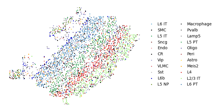
cluster = meta_data['celltype'].values
dt.plot_cell_type_ST(ad_st,mapping_colors,cluster)
Prediction of spatial CCC at the single-cell resolution.
Train the data using subgraph-based GAT and generate a prediction model.
The trained model can be used to predict intercellular communication mediated by other L-R interactions.
[27]:
lrpairs_train = {
    'ligand': ['Sst'],
    'receptor': ['Sstr2'],
    'species': ['Mouse']
}

lrpairs_train = pd.DataFrame(lrpairs_train)
lrpairs_train
[27]:
| ligand | receptor | species | |
|---|---|---|---|
| 0 | Sst | Sstr2 | Mouse |
[28]:
dt.File_Train(st_data, pathways, lrpairs_train, meta_data, species, LR_train = 'Sst_Sstr2',
              outdir =  Test_dir)
The training process may take some time. You can download trained models from github.
[29]:
dt.Train(data_name = 'Sst_Sstr2',data_path = Test_dir + '/data/',
    outdir = Test_dir + '/data/Sst_Sstr2/output',
    pretrained_embeddings = Test_dir + '/data/Sst_Sstr2/data_pca.emd',
    n_epochs = 50,ft_n_epochs=10)
 Loading graph...
DataSet Stats :
Number of Nodes 2399
Number of Edges 118483
Number of Node types 1
Number of relations 1
Graph with 2399 nodes and 118483 edges
2399 2
check torch.Size([2399, 128]) 2399
node2vec tensor torch.Size([2399, 128])
No. of nodes with pretrained embedding:  2399
No. edges in test data:  47795
***************PRETRAINING***************

 generate walks ...
no. of walks 19192
train ./test/single-cell//data//Sst_Sstr2/outdir/Sst_Sstr2_walks_train.txt
validate ./test/single-cell//data//Sst_Sstr2/outdir/Sst_Sstr2_walks_validate.txt
test ./test/single-cell//data//Sst_Sstr2/outdir/Sst_Sstr2_walks_test.txt

 Run model for pre-training ...

 Begin Training

Epoch: 0
MinLoss: 1000000.0, CurLoss: 7.9268
epoch time: (s) 31.95114231109619

Epoch: 10
MinLoss: 1000000.0, CurLoss: 7.8054
epoch time: (s) 30.530267000198364

Epoch: 20
MinLoss: 1000000.0, CurLoss: 7.7268
epoch time: (s) 31.17546510696411

Epoch: 30
MinLoss: 1000000.0, CurLoss: 7.291
epoch time: (s) 31.389280796051025

Epoch: 40
MinLoss: 1000000.0, CurLoss: 6.8481
epoch time: (s) 31.685405254364014

Best Epoch: 49
In GenericGraph link Prediction Generation
167282
Generating false edges by random false target
train
valid
test

 !!!!
4 4 Linear(in_features=512, out_features=512, bias=True)
Evaluating valid batch 0
Evaluating valid batch 100
Evaluating test batch 0
Evaluating test batch 100
Evaluating test batch 200

 Begin evaluation for link prediction...
----------------------In run_evaluation_main()------------
y_true.shape: (205503,), y_scores.shape: (205503,), y_pred.shape: (205503,)
workflow2 : ROC-AUC: 0.526741698940203, F1: 0.9194523062801193, AUC: 0.8823337862613925

Evaluation by edge type:
Performance on edge type:  to
y_true.shape: (47795,), y_scores.shape: (47795,), y_pred.shape: (47795,)
workflow2 : ROC-AUC: 0.5276606363036955, F1: 0.9191604204701374, PR-AUC: 0.8818182125782473
END
***************FINETUNING***************

 Run model for finetuning ...
4 4 Linear(in_features=512, out_features=512, bias=True)

 Begin Training
MinLoss: 1000000.0, CurLoss: 0.3276

Finetune epoch:  0
MinLoss:  0.3276
epoch time: (s) 645.191832780838
MinLoss: 1000000.0, CurLoss: 0.2839

Finetune epoch:  1
MinLoss:  0.2839
epoch time: (s) 636.3526470661163
MinLoss: 1000000.0, CurLoss: 0.2715

Finetune epoch:  2
MinLoss:  0.2715
epoch time: (s) 628.6298849582672
MinLoss: 1000000.0, CurLoss: 0.2617

Finetune epoch:  3
MinLoss:  0.2617
epoch time: (s) 632.8044881820679
MinLoss: 1000000.0, CurLoss: 0.2618

Finetune epoch:  4
MinLoss:  0.2618
epoch time: (s) 632.6420147418976
MinLoss: 1000000.0, CurLoss: 0.2585

Finetune epoch:  5
MinLoss:  0.2585
epoch time: (s) 630.1226873397827
MinLoss: 1000000.0, CurLoss: 0.2581

Finetune epoch:  6
MinLoss:  0.2581
epoch time: (s) 634.6195230484009
MinLoss: 1000000.0, CurLoss: 0.2575

Finetune epoch:  7
MinLoss:  0.2575
epoch time: (s) 635.4053466320038
MinLoss: 1000000.0, CurLoss: 0.2535

Finetune epoch:  8
MinLoss:  0.2535
epoch time: (s) 643.1755013465881
MinLoss: 1000000.0, CurLoss: 0.2555

Finetune epoch:  9
MinLoss:  0.2555
epoch time: (s) 623.6962542533875

Best Epoch: 8
Begin Testing
4 4 Linear(in_features=512, out_features=512, bias=True)
4 4 Linear(in_features=512, out_features=512, bias=True)
Evaluating test batch 0
Evaluating test batch 100
Evaluating test batch 200

 Begin evaluation for link prediction...
----------------------In run_evaluation_main()------------
y_true.shape: (205503,), y_scores.shape: (205503,), y_pred.shape: (205503,)
workflow3 : ROC-AUC: 0.9317243037944737, F1: 0.9304151455583637, AUC: 0.9899624449842547

Evaluation by edge type:
Performance on edge type:  to
y_true.shape: (47795,), y_scores.shape: (47795,), y_pred.shape: (47795,)
workflow3 : ROC-AUC: 0.9308336175971073, F1: 0.929916252125181, PR-AUC: 0.989772742741955
END
running time(seconds) on Sst_Sstr2 data: 11544.655077695847
Predicting cell-cell communication mediated by ``Apoe-Grm5``.
[30]:
lrpairs_pre = {
    'ligand': ['Apoe'],
    'receptor': ['Grm5'],
    'species': ['Mouse']
}

lrpairs_pre = pd.DataFrame(lrpairs_pre)
lrpairs_pre
[30]:
| ligand | receptor | species | |
|---|---|---|---|
| 0 | Apoe | Grm5 | Mouse |
[31]:
dt.File_Pre(st_data, pathways, lrpairs_pre, meta_data, species, LR_Pre = 'Apoe_Grm5',
              outdir =  Test_dir)
[32]:
dt.data_for_pre(st_data, data_dir = Test_dir +'/data/',
    LR_pre = 'Apoe_Grm5')
[33]:
dt.run_predict(data_name='Apoe_Grm5',data_path = Test_dir +'/data/',
    outdir = Test_dir +'/data/Apoe_Grm5/output',
    pretrained_embeddings = Test_dir +'/data/Apoe_Grm5/data_pca_pre.emd',
    model_path = Test_dir + '/data/Sst_Sstr2/output/finetune/results',
    best_id = 8, is_trained = True, model_name = Test_dir + '/Sst_Sstr2.model')
DataSet Stats :
Number of Nodes 2324
Number of Edges 111881
Number of Node types 1
Number of relations 1
check torch.Size([2324, 128]) 2256
node2vec tensor torch.Size([2324, 128])
4 4 Linear(in_features=512, out_features=512, bias=True)
Begin Predicting
Done
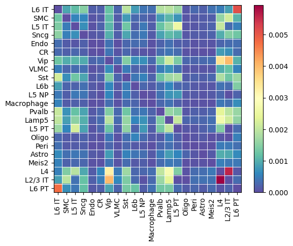
Visualize of the spatial CCC
Spatial distribution of cell types
Spatial cell-cell communication at single-cell resolution
Show Top 50 communication score for predticted cell-cell communication
[34]:
%matplotlib inline
import matplotlib.pyplot as plt
dt.plot_CCC_ST(ad_st, mapping_colors, cluster, st_data, ligand = 'Apoe',
    receptor = 'Grm5',CCC_label = Test_dir + '/data/Apoe_Grm5/predict_ccc.txt',
    sourcetype = 'L2/3 IT',targettype = 'L4',top_score = 50)
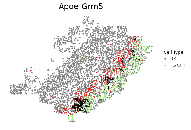
Cell-cell communication between cell types
[35]:
%matplotlib inline
import matplotlib.pyplot as plt
dt.plot_CCC_heatmap(cluster, st_data, ligand = 'Apoe', receptor = 'Grm5',
    CCC_label = Test_dir + '/data/Apoe_Grm5/predict_ccc.txt')
[ ]:
[ ]: